Hướng dẫn phát hiện vị trí khuyết điểm trên ảnh với Grad-CAM và Activation Map

by SDSRV · Published Tháng Chín 26, 2022 · Updated Tháng Chín 26, 2022

Xu hướng phát triển trong thời đại 4.0 liên tục đòi hỏi các nhà máy/ dây chuyền sản xuất phải nâng cấp về công nghệ sản xuất để nâng cao sản lượng và chất lượng sản phẩm. Bên cạnh các phương pháp kiểm tra tính năng sản phẩm, ngoại quan của các thành phẩm thường được kiểm tra bằng camera, thông qua các phương pháp xử lý ảnh và các mô hình học máy. Ở bài viết này, chúng tôi sẽ giới thiệu phương pháp phát hiện vị trí lỗi sản phẩm thông qua các mô hình phân loại ảnh (image classification) kết hợp với hai kĩ thuật phổ biến là Grad-CAM và Activation Map.

I. So sánh các phương pháp phát hiện khuyết điểm sản phẩm dựa trên ảnh

Việc phát hiện khuyết kiểm ngoại quan sản phẩm dựa trên ảnh có thể được thực hiện bằng nhiều kĩ thuật khác nhau, một số kĩ thuật phổ biến bao gồm:

Xử lý ảnh truyền thống & Học máy cơ bản
Sử dụng mô hình học sâu phát hiện đối tượng (object detection)
Sử dụng mô hình học sâu phân đoạn ảnh (image segmentation)
Sử dụng mô hình học sâu phân đoạn đối tượng (instance segmentation)
Sử dụng mô hình học sâu phân loại ảnh, kết hợp với cac phương pháp activation/attention map để xác định vị trí đối tượng

Ở phương pháp xử lý ảnh truyền thống, chúng ta sẽ áp dụng các kĩ thuật xử lý ảnh truyền thống như tìm biên đối tượng, tìm contour, phân đoạn ảnh dựa trên màu sắc, tính chất ảnh để tìm ra đối tượng là các khuyết điểm của ảnh. Ưu điểm của phương pháp này là không cần dữ liệu để huấn luyện các mô hình học máy và thường đòi hỏi chi phí tính toán thấp hơn. Tuy nhiên, phương pháp xử lý ảnh truyền thống thường bị ảnh hưởng bởi nhiễu nên gặp khó khăn khi phát hiện các đối tượng trong môi trường phức tạp hoặc có nhiều nhiễu. Nghiên cứu [2] là một ví dụ về việc sử dụng xử lý ảnh đơn thuần để tìm ra khuyết điểm trên ảnh, trong khi nghiên cứu [3] kết hợp thêm thuật toán học máy cổ điển là cây quyết định (decision tree).

**Luồng xử lý cho phương pháp 1: Xử lý ảnh + Học máy cơ bản**

Các phương pháp phát hiện đối tượng [4], [5] có khả năng phát hiện vùng bao hình chữ nhật bao quanh các khuyết điểm; các mô hình phân đoạn ảnh [6] và phân đoạn đối tượng [7] có thể dự đoán vị trí các khuyết điểm với độ chính xác đến từng điểm ảnh. Tuy vậy, các phương pháp này yêu cầu việc gán nhãn dữ liệu tương ứng (vùng bao, điểm ảnh), thường khá tốn công sức và chi phí.

**Luồng xử lý cho phương pháp 2, 3, 4: Ứng dụng học sâu cho phát hiện khuyết điểm**
**Hình ảnh được chỉnh sửa từ [7]**

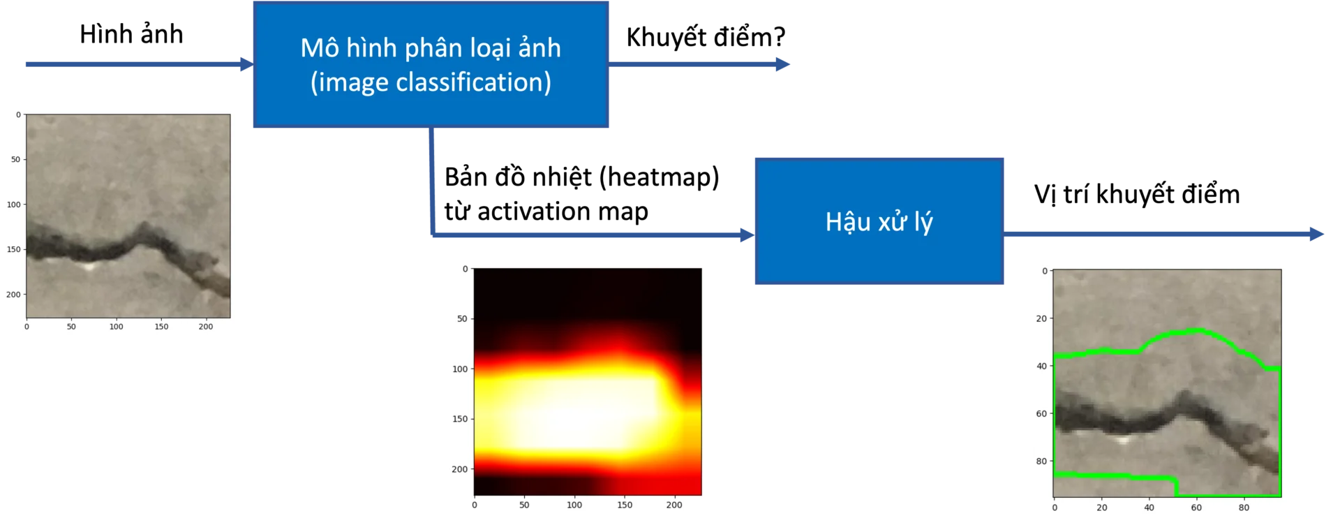
Phương pháp sử dụng mô hình phân loại hình ảnh kết hợp activation/attention map (5) được giới thiệu trong bài viết này có thể được coi là một giải pháp cân bằng giữa chi phí gán nhãn và kết quả đạt được. Việc gán nhãn chỉ yêu cầu phân loại các hình ảnh thành các lỗi / khuyết điểm khác nhau. Ví dụ, với bài toán phát hiện vết nứt trên bê tông, phương pháp này chỉ yêu cầu người dùng thu thập và phân loại ảnh thành 2 loại: chứa vết nứt và không chứa vết nứt. Sau khi huấn luyện mô hình, các kĩ thuật activation/attention map sẽ được sử dụng để xác định các vùng trong ảnh có ảnh hưởng nhất đến kết quả phân loại. Những vùng này thường là các đối tượng khuyết điểm cần xác định.

**Luồng xử lý cho phương pháp sử dụng mô hình phân loại ảnh kết hợp activation/attention map**

II. Phát hiện vết nứt vỡ trên bộ dữ liệu bê tông với Grad-CAM

Trong bài viết này, chúng tôi sẽ xây dựng mô hình cơ bản nhằm phát hiện khuyết điểm trên ảnh với bộ dữ liệu vết nứt bê tông Concrete Crack Images for Classification – Cung cấp bởi Özgenel, Çağlar Fırat (2019). Bộ dữ liệu này được thu thập từ METU Campus Buildings, bao gồm 20.000 hình ảnh chứa vết nứt bê tông và 20.000 ảnh không chứa vết nứt. Vị trí các vết nứt này chưa được gán nhãn rõ ràng. Chúng ta sẽ huấn luyện mô hình phân loại hình ảnh (chứa vết nứt / không chứa vết nứt) và sử dụng phương pháp Grad-CAM để định vị vết nứt tại mỗi ảnh.

Grad-CAM giúp xác định vị trí vết nứt thế nào? Ý tưởng của Grad-CAM dựa trên class activation map để xác định vị trí của đối tượng. Vùng ảnh chứa đối tượng cần tìm thường là vùng ảnh hưởng nhiều nhất đến kết quả dự đoán lớp, vì thế thường cho gradient mạnh nhất khi thực hiện lan truyền ngược (back proparation). Sau khi huấn luyện một mạng phân loại ảnh (chứa vết nứt / không chứa vết nứt), chúng ta đi tính toán lại gradient tại mỗi điểm lớp CNN (convolutional neural network) cuối cùng của mạng. Sự cập nhật của lớp cuối cùng này sẽ thể hiện vùng nào ảnh hưởng mạnh nhất đến kết quả phân loại. Kết quả này sẽ được sử dụng để khoanh vùng vết nứt.

1. Chuẩn bị dữ liệu

Trước tiên chúng ta cài đặt các gói cần thiết cho môi trường thí nghiệm:

!pip install tensorflow gdown imutils opencv-python matplotlib scipy Pillow PyYAML > /dev/null
# !pip install tensorflow-macos gdown imutils opencv-python matplotlib scipy Pillow PyYAML
 
import random
import shutil
import glob
import time
import os
import pathlib
 
import cv2
from imutils import paths
from IPython.display import display
from PIL import Image
import matplotlib.pyplot as plt
import matplotlib.cm as cm
import numpy as np
 
import tensorflow as tf
from tensorflow.keras.preprocessing.image import ImageDataGenerator

Bộ dữ liệu cần dùng đã được chúng tôi phân phối lại để có thể dễ dàng tải về hơn với lệnh gdown.

!gdown 1A-XotBf-dt8JqzH_xiOFVPFWjHs2Y2ac
!ls

Downloading...

Sau khi tải về và giải nén dữ liệu, chúng ta sẽ thu được bộ dữ liệu trong thư mục concrete_crack_dataset, với cấu trúc như bên dưới.

Thư mục Negative chứa các ảnh không có vết nứt, thư mục Positive chứa các ảnh bê tông có vết nứt.

+ concrete_crack_dataset    
    + raw
        + Negative: 20k ảnh không chứa vết nứt
        + Positive: 20k ảnh chứa vết nứt

!ls concrete_crack_dataset/raw

Negative  Positive

Chúng ta cùng xem qua một vài ảnh trong bộ dữ liệu này:

def show_images(path):
    """Visualize images from path"""
    all_img_paths = list(paths.list_images(path))
    plt.figure(figsize=(15,15))
    for i in range(25):
        image_path = np.random.choice(all_img_paths)
        image = plt.imread(image_path)
        image = cv2.resize(image, (96, 96))
        label = os.path.basename(pathlib.Path(image_path).parent)
        plt.subplot(5,5,i+1)
        plt.xticks([])
        plt.yticks([])
        plt.grid(True)
        plt.imshow(image)
        plt.xlabel(label + " " + os.path.basename(image_path)[:8])
    plt.show()
show_images("concrete_crack_dataset/raw")

Chia dữ liệu: Để phục vụ huấn luyện mô hình, chúng ta sẽ chia dữ liệu làm hai phần nhỏ:

Tập huấn luyện (training set): 80%
Tập giám sát (validation set): 20%

Việc chia dữ liệu sẽ đảm bảo các lớp (Positive/Negative) phân bố đều trong các tập dữ liệu con.

+ concrete_crack_dataset
    + raw
        + Negative: 20k ảnh không chứa vết nứt
        + Positive: 20k ảnh chứa vết nứt
    + train: Tập huấn luyện - 80% dữ liệu
        + Negative
        + Positive
    + val: Tập giám sát - 20% dữ liệu
        + Negative
        + Positive

def split_data(input_folder, train_folder, val_folder, train_ratio):
    """Split data into training and validation sets"""
    assert(train_ratio >= 0 and train_ratio <= 1.0)
    pathlib.Path(train_folder).mkdir(parents=True, exist_ok=True)
    pathlib.Path(val_folder).mkdir(parents=True, exist_ok=True)
 
    files = list(os.listdir(input_folder))
    random.seed(42)
    random.shuffle(files)
 
    num_files = len(files)
    num_train_files = int(num_files * train_ratio)
 
    train_files = files[:num_train_files]
    val_files = files[num_train_files:]
 
    print(f"Training images: {len(train_files)}; Validation images: {len(val_files)}")
 
    for f in train_files:
        shutil.copy(os.path.join(input_folder, f), os.path.join(train_folder, f))
    for f in val_files:
        shutil.copy(os.path.join(input_folder, f), os.path.join(val_folder, f))
 
train_ratio = 0.8
raw_dir = "concrete_crack_dataset/raw"
train_dir = "concrete_crack_dataset/train"
val_dir = "concrete_crack_dataset/val"
for cls in ["Positive", "Negative"]:
    print(f"Class: {cls}")
    split_data(
        f"{raw_dir}/{cls}",
        f"{train_dir}/{cls}",
        f"{val_dir}/{cls}",
        train_ratio,
    )

Class: Positive
Training images: 16000; Validation images: 4000
Class: Negative
Training images: 16000; Validation images: 4000

2. Huấn luyện mô hình

Việc xây dựng và huấn luyện mô hình sẽ được thực hiện trên Tensorflow/Keras.

Nạp dữ liệu huấn luyện:

Tensorflow/Keras đã hỗ trợ cơ bản việc nạp dữ liệu cho huấn luyện mô hình phân loại hình ảnh. Bằng việc sử dụng ImageDataGenerator, chúng ta có thể thêm các thao tác chuyển đổi, tăng cường dữ liệu. Ở đây, chúng tôi dùng tham số rescale để chuyển đổi dữ liệu các điểm ảnh về đoạn [0, 1]; horizontal_flip, vertical_flip được sử dụng nhằm tăng cường dữ liệu. Dữ liệu sẽ được nạp lên thông qua data loader của Keras, tạo thông qua hàm flow_from_directory().

batch_size = 16
train_aug = ImageDataGenerator(rescale=1/255.,
                                horizontal_flip=True,
                                vertical_flip=True)
val_aug = ImageDataGenerator(rescale=1/255.,
                             horizontal_flip=False,
                             vertical_flip=False)
 
print("Training set")
train_gen = train_aug.flow_from_directory(train_dir,
    class_mode="categorical",
    target_size=(224, 224),
    color_mode="rgb",
    shuffle=True,
    batch_size=batch_size
)
 
print("Validation set")
val_gen = val_aug.flow_from_directory(val_dir,
    class_mode="categorical",
    target_size=(224, 224),
    color_mode="rgb",
    shuffle=False,
    batch_size=batch_size
)
num_classes = len(train_gen.class_indices.keys())
print("Set number of classes to {}".format(num_classes))

Training setFound 32000 images belonging to 2 classes.
Validation set
Found 8000 images belonging to 2 classes. Set number of classes to 2

# Get the class labels and export to labels.txt
print("Training set:", train_gen.class_indices)
print("Validation set:", val_gen.class_indices)
labels = '\n'.join(sorted(train_gen.class_indices.keys()))
with open('labels.txt', 'w') as f: 
f.write(labels)

Training set: {'Negative': 0, 'Positive': 1}
Validation set: {'Negative': 0, 'Positive': 1}

Xây dựng mô hình:

Mô hình phân loại ảnh sẽ được xây dựng dựa trên MobileNetV2 – một mô hình phân loại ảnh tập trung vào tối ưu hoá tốc độ xử lý cho các thiết bị di động. Phần khung xương (backbone) của mạng sẽ lấy kiến trúc có sẵn trong framework Keras, kết hợp trọng số có sẵn được huấn luyện trên tập imagenet. Lớp Dense cuối cùng sẽ thực hiện phân loại ảnh thành các lớp khác nhau (ở đây num_classs=2).

def build_model():
    extractor = tf.keras.applications.MobileNetV2(weights="imagenet", include_top=False, input_shape=(224, 224, 3))
    extractor.trainable = True
    class_head = extractor.output
    class_head = tf.keras.layers.GlobalAveragePooling2D()(class_head)
    class_head = tf.keras.layers.Dropout(0.2)(class_head)
    class_head = tf.keras.layers.Dense(num_classes, activation="softmax")(class_head)
    classifier = tf.keras.models.Model(inputs=extractor.input, outputs=class_head)
    return classifier

Huấn luyện:

Quá trình huấn luyện mô hình sẽ trải qua 5 epochs, việc chọn lựa mô hình tốt nhất được dựa trên độ chính xác trên tập giám sát. Trong quá trình huấn luyện, các mô hình có độ chính xác (accuracy) tốt nhất trên tập giám sát sẽ được lưu lại với tên “best_model_checkpoint.h5”.

# Training parameters
num_epochs = 5
 
classification_model = build_model()
classification_model.compile(loss="categorical_crossentropy",
                          optimizer=tf.keras.optimizers.Adam(0.0001),
                          metrics=["accuracy"])
 
# Setup a callback to save the best model
best_model_path = "best_model_checkpoint.h5"
model_checkpoint_callback = tf.keras.callbacks.ModelCheckpoint(
    filepath=best_model_path,
    save_weights_only=False,
    monitor='val_accuracy',
    mode='max',
    save_best_only=True)
 
start = time.time()
train_steps = train_gen.samples // batch_size
val_steps = val_gen.samples // batch_size
history = classification_model.fit(train_gen,
    steps_per_epoch=train_steps,
    validation_data=val_gen,
    validation_steps=val_steps,
    epochs=num_epochs,
    callbacks=[model_checkpoint_callback]
)
print("Total training time: ", time.time() - start)


Epoch 1/5
2000/2000 [==============================] - 158s 77ms/step - loss: 0.0217 - accuracy: 0.9933 - val_loss: 0.0452 - val_accuracy: 0.9824
Epoch 2/5
2000/2000 [==============================] - 153s 76ms/step - loss: 0.0088 - accuracy: 0.9974 - val_loss: 0.0087 - val_accuracy: 0.9987
Epoch 3/5
2000/2000 [==============================] - 153s 77ms/step - loss: 0.0058 - accuracy: 0.9982 - val_loss: 0.0065 - val_accuracy: 0.9986
Epoch 4/5
2000/2000 [==============================] - 154s 77ms/step - loss: 0.0066 - accuracy: 0.9978 - val_loss: 0.0122 - val_accuracy: 0.9979
Epoch 5/5
2000/2000 [==============================] - 154s 77ms/step - loss: 0.0067 - accuracy: 0.9982 - val_loss: 0.0050 - val_accuracy: 0.9985
Total training time:  771.1618840694427

# Plot training graph
N = len(history.history["loss"])
plt.figure()
plt.plot(np.arange(0, N), history.history["loss"], label="train_loss")
plt.plot(np.arange(0, N), history.history["val_loss"], label="val_loss")
plt.plot(np.arange(0, N), history.history["accuracy"], label="train_acc")
plt.plot(np.arange(0, N), history.history["val_accuracy"], label="val_acc")
plt.title("Training Loss and Accuracy")
plt.xlabel("Epoch #")
plt.ylabel("Loss/Accuracy")
plt.legend(loc="lower left")
plt.show()

Sau khi huấn luyện, ta nạp lại checkpoint tốt nhất và thực hiện kiểm thử lại trên tập giám sát.

classification_model = tf.keras.models.load_model("best_model_checkpoint.h5")
eval_result = classification_model.evaluate(val_gen)
val_accuracy = eval_result[1]
print("Model accuracy on validation set: {}".format(val_accuracy))

500/500 [==============================] - 8s 14ms/step - loss: 0.0087 - accuracy: 0.9987
Model accuracy on validation set: 0.9987499713897705

3. Tính toán Grad-CAM

Thuật toán Grad-CAM sẽ sử dụng gradient của lớp tích chập cuối để tạo ra một bản đồ nhiệt (heatmap), thể hiện tầm quan trọng của mỗi vùng ảnh trong việc quyết định lớp đầu ra. Dưới đây, ta sẽ sử dụng hàm make_gradcam_heatmap() để tính toán đầu ra cho bản đồ nhiệt. Hàm get_prediction_with_heatmap() được sử dụng để trả về cả dự đoán phân lớp và bản đồ nhiệt cho một hình ảnh đầu vào.

def make_gradcam_heatmap(img_array, model, last_conv_layer_name, pred_index=None):
    """Get Grad-CAM heatmap from model"""
    # First, we create a model that maps the input image to the activations
    # of the last conv layer as well as the output predictions
    grad_model = tf.keras.models.Model(
        [model.inputs], [model.get_layer(last_conv_layer_name).output, model.output]
    )
 
    # Then, we compute the gradient of the top predicted class for our input image
    # with respect to the activations of the last conv layer
    with tf.GradientTape() as tape:
        last_conv_layer_output, preds = grad_model(img_array)
        if pred_index is None:
            pred_index = tf.argmax(preds[0])
        class_channel = preds[:, pred_index]
 
    # This is the gradient of the output neuron (top predicted or chosen)
    # with regard to the output feature map of the last conv layer
    grads = tape.gradient(class_channel, last_conv_layer_output)
 
    # This is a vector where each entry is the mean intensity of the gradient
    # over a specific feature map channel
    pooled_grads = tf.reduce_mean(grads, axis=(0, 1, 2))
 
    # We multiply each channel in the feature map array
    # by "how important this channel is" with regard to the top predicted class
    # then sum all the channels to obtain the heatmap class activation
    last_conv_layer_output = last_conv_layer_output[0]
    heatmap = last_conv_layer_output @ pooled_grads[..., tf.newaxis]
    heatmap = tf.squeeze(heatmap)
 
    # For visualization purpose, we will also normalize the heatmap between 0 & 1
    heatmap = tf.maximum(heatmap, 0) / tf.math.reduce_max(heatmap)
    return heatmap.numpy()
 
def preprocess_img(img):
    """Preprocess for OpenCV python image"""
    img = cv2.resize(img, (224, 224))
    img = cv2.cvtColor(img, cv2.COLOR_BGR2RGB)
    img = img / 255.0
    return img
 
def get_prediction_with_heatmap(model, origin_img):
    """Get prediction with heatmap output"""
    origin_img_height, origin_img_width = origin_img.shape[:2]
    img = preprocess_img(origin_img)
    img_array = np.expand_dims(img, axis=0)
 
    # Print what the top predicted class is
    preds = model.predict(img_array, verbose=0)
 
    # Remove last layer's softmax
    model.layers[-1].activation = None
 
    def find_target_layer(model):
        # attempt to find the final convolutional layer in the network
        # by looping over the layers of the network in reverse order
        for layer in reversed(model.layers):
            # check to see if the layer has a 4D output
            if len(layer.output_shape) == 4:
                return layer.name
 
        print(f"Last Conv. Layer: {layer.name}")
 
        # otherwise, we could not find a 4D layer so the GradCAM
        # algorithm cannot be applied
        raise ValueError("Could not find 4D layer. Cannot apply GradCAM.")
 
    last_conv_layer_name = find_target_layer(model)
 
    # Generate class activation heatmap
    heatmap = make_gradcam_heatmap(img_array, model, last_conv_layer_name)
    heatmap = cv2.resize(heatmap, (origin_img_width, origin_img_height))
 
    return preds[0], heatmap

4. Trực quan hóa kết quả

Đoạn mã dưới đây sẽ chạy mô hình trên một hình ảnh lấy từ tập giám sát, tính toán kết quả (prediction) và bản đồ nhiệt từ Grad-CAM. Tiếp đó hàm cv2.findContours() của OpenCV sẽ được sử dụng để tìm vùng bao quanh các điểm bất thường trong ảnh (ảnh hưởng nhiều nhất tới kết quả dự đoán). Hình ảnh ban đầu, hình ảnh bản đồ nhiệt và hình vẽ vùng bao cuối cùng sẽ được thể hiện ngang hàng nhau.

best_model_path = "best_model_checkpoint.h5"
model = tf.keras.models.load_model(best_model_path)
all_img_paths = sorted(list(paths.list_images("concrete_crack_dataset/val")))
 
def find_contours_from_heatmap(preds, heatmap):
    """Find contours"""
    if preds[1] > 0.5: # Cracked
        heatmap[heatmap < 40] = 0
        contours, hierarchy = cv2.findContours(heatmap, cv2.RETR_TREE, cv2.CHAIN_APPROX_SIMPLE)
        return contours
    return []
 
def predict_and_show(all_img_paths):
    """Get prediction and show visualization"""
    np.random.seed(101)
    img_path = np.random.choice(all_img_paths)
    origin_img = cv2.imread(img_path)
     
    # Show original image
    f, axarr = plt.subplots(1,3)
    axarr[0].imshow(Image.open(img_path))
     
    preds, heatmap = get_prediction_with_heatmap(model, origin_img)
    print("Prediction:", preds)
    heatmap = heatmap * 255.0
    heatmap = heatmap.astype(np.uint8)
     
    # Show heatmap
    axarr[1].imshow(heatmap, cmap="hot")
 
    # Draw image
    draw = origin_img.copy()
    contours = find_contours_from_heatmap(preds, heatmap)
    cv2.drawContours(draw, contours, -1, (0, 255, 0), 3)
 
    # Show contours
    draw = cv2.resize(draw, (96, 96))
    draw = cv2.cvtColor(draw, cv2.COLOR_BGR2RGB)
    axarr[2].imshow(draw)
     
predict_and_show(all_img_paths)

Prediction: [2.5866856e-32 1.0000000e+00]

Sau khi dự đoán một hình ảnh, chúng ta cùng chạy dự đoán trên một loạt ảnh để thử nghiệm kết quả mô hình.

best_model_path = "best_model_checkpoint.h5"
model = tf.keras.models.load_model(best_model_path)
 
def predict_and_show_many(all_img_paths):
    """Get prediction and show visualization for a batch of images from dataset"""
    plt.figure(figsize=(15,15))
    np.random.seed(42)
    for i in range(25):
        img_path = np.random.choice(all_img_paths)
        origin_img = cv2.imread(img_path)
        preds, heatmap = get_prediction_with_heatmap(model, origin_img)
        heatmap = heatmap * 255.0
        heatmap = heatmap.astype(np.uint8)
 
        # Draw image
        draw = origin_img.copy()
        contours = find_contours_from_heatmap(preds, heatmap)
        cv2.drawContours(draw, contours, -1, (0, 255, 0), 3)
             
        draw = cv2.resize(draw, (96, 96))
        draw = cv2.cvtColor(draw, cv2.COLOR_BGR2RGB)
     
        label = "Defected" if preds[1] > 0.5 else "Good"
        plt.subplot(5,5,i+1)
        plt.xticks([])
        plt.yticks([])
        plt.grid(True)
        plt.imshow(draw)
        plt.xlabel(label + " " + os.path.basename(img_path)[:8])
    plt.show()
     
predict_and_show_many(all_img_paths)

Như chúng ta đã thấy, việc tính toán vị trí vết nứt thông qua thuật toán Grad-CAM tương đối tốt. Tuy nhiên để tính lan truyền ngược (backpropagation) một cách dễ dàng, mô hình cần được thực thi bằng một framework huấn luyện mô hình (Tensorflow, Pytorch, …). Tất nhiên chúng ta cũng có thể tính toán lại một cách thủ công. Ở phần này, ta sẽ tham khảo một hướng tiếp cận khác – attention map. Phương pháp này sử dụng chính lớp convolution ở cuối để xác định vị trí đối tượng, không cần đến việc tính toán gradient như Grad-CAM.

Phần mã nguồn bên dưới sẽ thêm nhánh heatmap (bản đồ nhiệt) vào mô hình phân loại đã huấn luyện phía trên. Đầu ra heatmap sẽ được tính toán từ lớp tích chập (convolution) cuối cùng. Kết hợp với số bước xử lý lọc và tìm vùng bao (contour) , ta sẽ ra được vị trí vết nứt.

def build_model_attention(num_classes, input_shape):
    """Build attention model - Output the last convolution layer as heatmap"""
    extractor = tf.keras.applications.MobileNetV2(weights="imagenet", include_top=False, input_shape=(224, 224, 3))
    extractor.trainable = True
 
    class_head = extractor.output
    class_head = tf.keras.layers.GlobalAveragePooling2D()(class_head)
    class_head = tf.keras.layers.Dropout(0.2)(class_head)
    class_head = tf.keras.layers.Dense(num_classes, activation="softmax")(class_head)
     
    heatmap = tf.math.reduce_sum(
        extractor.output, axis=-1, keepdims=True
    )
    heatmap = tf.maximum(heatmap, 0) / tf.math.reduce_max(heatmap)
     
    classifier = tf.keras.models.Model(inputs=extractor.input, outputs=[class_head, heatmap])
    return classifier
 
 
model = build_model_attention(2, (224, 224))
model.load_weights("best_model_checkpoint.h5")

Kết quả của phương pháp này cũng được trực quan hóa với các bước như phần trước.

def predict_and_show_attention(all_img_paths):
    """Predict and show attention map"""
    plt.figure(figsize=(15,15))
    np.random.seed(42)
    for i in range(25):
        img_path = np.random.choice(all_img_paths)
        origin_img = cv2.imread(img_path)
 
        origin_img_height, origin_img_width = origin_img.shape[:2]
        img = preprocess_img(origin_img)
        img_array = np.expand_dims(img, axis=0)
        preds, heatmap = model.predict(img_array, verbose=0)
        preds = preds[0]
        heatmap = heatmap[0]
        heatmap = cv2.resize(heatmap, (origin_img_width, origin_img_height))
        heatmap = heatmap * 255.0
        heatmap = heatmap.astype(np.uint8)
 
        contours = find_contours_from_heatmap(preds, heatmap)
         
        draw = origin_img.copy()
        cv2.drawContours(draw, contours, -1, (0, 255, 0), 3)
 
        draw = cv2.resize(draw, (96, 96))
        draw = cv2.cvtColor(draw, cv2.COLOR_BGR2RGB)
     
        label = "Defected" if preds[1] > 0.5 else "Good"
        plt.subplot(5,5,i+1)
        plt.xticks([])
        plt.yticks([])
        plt.grid(True)
        plt.imshow(draw)
        plt.xlabel(label + " " + os.path.basename(img_path)[:8])
    plt.show()
     
predict_and_show_attention(all_img_paths)

IV. Kết luận

Phương pháp xác định khuyết điểm sản phẩm thông qua mô hình phân loại ảnh kết hợp activation/attention map cho hiệu quả tương đối tốt với các bộ dữ liệu không quá phức tạp. Với ưu điểm về việc tối thiểu hoá quá trình gán nhãn dữ liệu, phương pháp này sẽ tiết kiệm nhiều thời gian và công sức trong việc phát triển sản phẩm. Tuy vậy, vị trí các khuyết điểm được tạo ra bằng phương pháp này thường khó kiểm soát về chất lượng và độ chính xác cũng thường thấp hơn các mô hình phân đoạn (image segmentation, instance segmentation) và phát hiện vật thể (object detection) nếu được gán nhãn đầy đủ. Chính vì thế, việc lựa chọn mô hình và phương pháp xử lý sẽ phụ thuộc vào yêu cầu bài toán hay vấn đề cần được giải quyết trong thực tế. Chúng tôi hi vọng đã cung cấp được kiến thức hữu ích cho các bạn về một hướng tiếp cận trong bài toán phát hiện khuyết điểm.